Answers to Revision Exercises
Revision Exercises 1
Q1.
What is the length of (total number of base-pairs in) the Schistosoma mansoni mitochondrial genome (NCBI accession NC_002545), and how many As, Cs, Gs and Ts does it contain?
To do this, you need to go to the www.ncbi.nlm.nih.gov website and type the S. mansoni mitochondrial genome (accession NC_002545) in the search box, and press ‘Search’.
On the search results page, you should see ‘1’ beside the word ‘Nucleotide’, meaning that there was one hit to a sequence record in the NCBI Nucleotide database, which contains DNA and RNA sequences. If you click on the word ‘Nucleotide’, it will bring you to the sequence record, which should be the NCBI sequence record for the S.mansoni mitochondrial genome (ie. for accession NC_002545).
To save the sequence as FASTA-format file, click on ‘Send’ at the top right of the page, and choose ‘File’, then select ‘FASTA’ from the drop-down list labelled ‘Format’, then click ‘Create File’. Save the file with a name that you will remember (eg. “smansoni.fasta”) in your “My Documents” folder.
You can then read the sequence into R by typing:
> library("seqinr")                                 # load the SeqinR R package
> smansoni <- read.fasta(file="smansoni.fasta")     # read in the sequence file
> smansoniseq <- smansoni[[1]]                      # get the sequence
> length(smansoniseq)                               # get the length of the sequence
  [1] 14415
> table(smansoniseq)                                # get the number of As, Cs, Gs, Ts
  smansoniseq
    a    c    g    t
  3654 1228 3307 6226
Thus, the mitochondrial genome is 14415 bases long, and consists of 3654 As, 1228 Cs, 3307 Gs and 6226 Ts.
Note that, as far as I know, it is not possible to retrieve the sequence for accession NC_002545 directly using the “query()” function in SeqinR, because the S. mansoni mitochondrial genome sequence does not seem to be stored in any of the ACNUC sub-databases.
Q2.
What is the length of the Brugia malayi mitochondrial genome (NCBI accession NC_004298), and how many As, Cs, Gs and Ts does it contain?
To do this, you need to go to the www.ncbi.nlm.nih.gov website and type the B. malayi mitochondrial genome (accession NC_004298) in the search box, and press ‘Search’.
As in Q1, go to the NCBI record for the sequence, and save the sequence in a FASTA format file, for example, called “bmalayi.fasta”.
Then read the sequence into R, and get its length and composition by typing:
> bmalayi <- read.fasta(file="bmalayi.fasta")       # read in the sequence file
> bmalayiseq <- bmalayi[[1]]                        # get the sequence
> length(bmalayiseq)                                # get the length of the sequence
  [1] 13657
> table(bmalayiseq)                                 # get the number of As, Cs, Gs, Ts
  bmalayiseq
   a    c    g    t
  2950 1054 2297 7356
The sequence is 13657 bases long, and consists of 2950 As, 1054 Cs, 2297 Gs and 7356 Ts.
Note that, as far as I know, it is not possible to retrieve the sequence for accession NC_004298 directly using the “query()” function in SeqinR, because the B. malayi mitochondrial genome sequence does not seem to be stored in any of the ACNUC sub-databases.
Q3.
What is the probability of the Brugia malayi mitochondrial genome sequence (NCBI accession NC_004298), according to a multinomial model in which the probabilities of As, Cs, Gs and Ts (pA, pC, pG, and pT) are set equal to the fraction of As, Cs, Gs and Ts in the Schistosoma mansoni mitochondrial genome?
First we can calculate the frequencies of A, C, G and T in the S. mansoni mitochondrial sequence. We can do this by making a table of the counts of As, Cs, Gs and Ts, and dividing the counts of the bases by the total sequence length to get frequencies:
> mytable <- table(smansoniseq)
> mytable
    a    c    g    t
  3654 1228 3307 6226
> mytable <- mytable/length(smansoniseq) # Divide the counts by the sequence length, to get frequencies
> mytable
     a          c          g          t
  0.25348595 0.08518904 0.22941381 0.43191120
> freqA <- mytable[["a"]]                # Get the frequency of As
> freqC <- mytable[["c"]]                # Get the frequency of Cs
> freqG <- mytable[["g"]]                # Get the frequency of Gs
> freqT <- mytable[["t"]]                # Get the frequency of Ts
> probabilities <- c(freqA,freqC,freqG,freqT) # Make a vector containing the frequencies of As,Cs,Gs,Ts
> probabilities
  [1] 0.25348595 0.08518904 0.22941381 0.43191120
First we need to make a function to calculate the probability of a sequence, given a particular multinomial model (with a certain pA, pC, pG, pT). To do this, we can write the following R function “multinomialprob()”:
> multinomialprob <- function(mysequence, probabilities)
  {
      nucleotides   <- c("A", "C", "G", "T") # Define the alphabet of nucleotides
      names(probabilities) <- nucleotides
      mysequence    <- toupper(mysequence)# Convert the sequence to uppercase letters
      seqlength     <- length(mysequence) # Get the length of the input sequence
      seqprob       <- numeric()          # Make a variable to hold to probability of the whole sequence
      for (i in 1:seqlength)              # For each letter in the input sequence
      {
         nucleotide <- mysequence[i]      # Find the ith nucleotide in the sequence
         # Calculate the probability of the ith nucleotide in the sequence
         nucleotideprob <- probabilities[nucleotide]
         # The probability of the whole sequence is calculated by multiplying together
         # the probabilities of the nucleotides at each sequence position
         if (i == 1) { seqprob <- nucleotideprob[[1]]           }
         else        { seqprob <- seqprob * nucleotideprob[[1]] }
      }
      # Return the value of the probability of the whole sequence
      return(seqprob)
  }
The function multinomialprob() takes as its arguments (inputs) a vector that contains the DNA sequence, and a vector containing the probabilities pA, pC, pG, and pT.
You will need to copy and paste this function into R to use it. You can then use it to calculate the probability of the B. malayi mitochondrial sequence, using a multinomial model where pA, pC, pG, pT are set equal to the fraction of As, Cs, Gs, and Ts in the S. mansoni mitohondrial sequence (which we have already stored in the vector probabilities, see above):
> multinomialprob(bmalayiseq, probabilities)
  0
In this case, the probability is so small that it is effectively zero.
Q4.
What are the top three most frequent 4-bp words (4-mers) in the genome of the bacterium Chlamydia trachomatis strain D/UW-3/CX (NCBI accession NC_000117), and how many times do they occur in its sequence?
To do this, you need to go to the www.ncbi.nlm.nih.gov website and type the C. trachomatis D/UW-3/CX genome (accession NC_000117) in the search box, and press ‘Search’.
As in Q1, go to the NCBI record for the sequence, and save the sequence in a FASTA format file, for example, called “ctrachomatis.fasta”.
Alternatively, you can retrieve the sequence using the SeqinR package. The sequence is a fully sequenced bacterial genome, so is in the ACNUC sub-database called “bacterial”. Thus, we type in R:
> choosebank("bacterial")                                # select the ACNUC sub-database to search
> query("ctrachomatis", "AC=NC_000117")                  # specify the query
> ctrachomatisseq <- getSequence(ctrachomatis$req[[1]])  # get the sequence
> closebank()                                            # close the connection to the ACNUC sub-database
We can now find the most frequent 4-bp words in the sequence by using the “count()” function from SeqinR:
> mytable <- count(ctrachomatisseq, 4)                   # get the count for each 4-bp word
> sort(mytable)                                          # sort the 4-bp words, by the number of occurrences of each word
  ccgg  cggg  ggcc  cccg  cgcg  cggc  gccg  cgcc  ggcg  cggt  gccc  cacg  gggc
  1180  1198  1206  1215  1287  1321  1334  1407  1435  1481  1512  1520  1537
  cgtg  accg  ggtc  gacc  cgac  gtcg  gcgg  ccgc  acgg  gacg  cgtc  ccgt  gtac
  1541  1545  1558  1567  1606  1647  1658  1678  1716  1750  1786  1802  1802
  ...
  agag  agct  ctct  tatt  cttc  tttg  caaa  gaag  ttta  taaa  attt  aaat  tttc
  6836  6860  6937  6946  7234  7280  7289  7353  7671  7731  8100  8144  8462
  gaaa  aaag  cttt  tctt  aaga  ttct  agaa  tttt  aaaa
  8563  9099  9199 10060 10069 10492 10581 14021 14122
The three most frequent 4-bp words are “aaaa” (14122 occurrences), “tttt” (14021 occurrences) and “agaa” (10581 occurrences).
Q5.
Write an R function to generate a random DNA sequence that is n letters long (that is, n bases long) using a multinomial model in which the probabilities pA, pC, pG, and pT are set equal to the fraction of As, Cs, Gs and Ts in the Schistosoma mansoni mitochondrial genome.
In Q3 above, we stored the frequencies of A, C, G and T in the S. mansoni mitochondrial genome in a vector called probabiltiies:
> probabilities
  [1] 0.25348595 0.08518904 0.22941381 0.43191120
The R function “generateSeqWithMultinomialModel()” below is an R function for generating a random sequence with a multinomial model, where the probabilities of the different letters are set equal to the fraction of As, Cs, Gs, and Ts in the S. mansoni mitochondrial genome (ie. with vector probabilities as its input):
> generateSeqWithMultinomialModel <- function(n, probabilities)
  {
     # Define the letters in the alphabet
     letters <- c("A", "C", "G", "T")
     # Make a random sequence of length n letters, using the multinomial model with probabilities "probabilities"
     seq <- sample(letters, n, rep=TRUE, prob=probabilities) # Sample with replacement
     # Return the sequence
     return(seq)
  }
To use this function to generate a 10-bp random sequence, using vector probabilities as input, we would type:
> generateSeqWithMultinomialModel(10, probabilities)
  [1] "T" "A" "T" "G" "T" "G" "G" "A" "G" "G"
Each time we call the function, it will create a slightly different 10-bp sequence:
> generateSeqWithMultinomialModel(10, probabilities)
  [1] "A" "G" "T" "A" "G" "G" "T" "T" "T" "T"
> generateSeqWithMultinomialModel(10, probabilities)
  [1] "C" "G" "A" "T" "A" "T" "G" "T" "T" "A"
Q6.
Give an example of using your function from Q5 to calculate a random sequence that is 20 letters long, using a multinomial model with pA =0.28, pC =0.21, pG =0.22, and pT =0.29.
First we need to define a vector myprobabilities containing the probabilities of A, C, G, and T:
> myprobabilities <- c(0.28, 0.21, 0.22, 0.29)
Then we can use the function “generateSeqWithMultinomialModel()” to calculate a 20-bp random sequence, using the vector myprobabilities as its input:
> generateSeqWithMultinomialModel(20, myprobabilities)
  [1] "C" "C" "G" "A" "T" "A" "T" "C" "C" "G" "C" "C" "T" "G" "A" "G" "T" "T" "T"
  [20] "C"
Q7.
How many protein sequences from rabies virus are there in the NCBI Protein database?
To do this, you need to go to the www.ncbi.nlm.nih.gov website and select ‘Protein’ from the drop-down box above the search box.
Then type “rabies virus”[ORGN] in the search box, and press ‘Search’.
On the results page, it should say “Results: 1 to 20 of 11768”, meaning that there are 11768 protein sequences from rabies virus in the database [as of 16-Jun-2011]. Note that if you carry out this search at a later date, you may find more sequences, as the database is growing all the time.
Q8.
What is the NCBI accession for the Mokola virus genome?
To do this, you need to go to the www.ncbi.nlm.nih.gov website and select ‘Genome’ from the drop-down box above the search box.
Then type “Mokola virus”[ORGN] in the search box, and press ‘Search’.
You should get a hit to accession NC_006429, the Mokola virus genome sequence.
Note that alternatively you can go to the www.ncbi.nlm.nih.gov website, and type “Mokola virus”[ORGN] in the search box, and press ‘Search’. On the results page, you will see lots of hits to the Nucleotide and Protein databases, and 1 hit to the Genome database. If you click on the 1 hit beside “Genome”, it will bring you to accession NC_006429, the Mokola virus genome sequence.
Revision Exercises 2
Q1.
Use the dotPlot() function in the SeqinR R package to make a dotplot of the rabies virus phosphoprotein and Mokkola virus phosphoprotein, using a windowsize of 10 and threshold of 5.
First we need to retrieve the rabies virus phosphoprotein (UniProt P06747) and Mokola virus phosphoprotein (UniProt P0C569) sequences from UniProt, which we can do using SeqinR:
> library("seqinr")                                      # load the SeqinR package
> choosebank("swissprot")                                # select the ACNUC sub-database to search
> query("rabies", "AC=P06747")                           # specify the query
> rabiesseq <- getSequence(rabies$req[[1]])              # get the sequence
> query("mokola", "AC=P0C569")                           # specify the query
> mokolaseq <- getSequence(mokola$req[[1]])              # get the sequence
> closebank()                                            # close the connection to the ACNUC sub-database
If you look at the help page of the dotPlot function (by typing “help(dotPlot)”), you will see that the windowsize can be specified using the “wsize” argument and the threshold can be specified using the “nmatch” argument.
We can therefore use dotPlot() to make a dotplot of the two proteins, using a windowsize of 10 and a threshold of 5, by typing:
> dotPlot(mokolaseq,rabiesseq,wsize=10,nmatch=5)
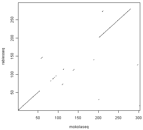
You can see that there is a region of similarity that covers about 60-70 amino acids at the start of the two proteins, then there is a region of similarity from about 210-280 in each of the two proteins. There is also a weak amount of similarity in a region from about 85-100 in the two proteins.
Q2.
Use the function makeDotPlot1 to make a dotplot of the rabies virus phosphoprotein and the Mokola virus phosphoprotein, setting the argument “dotsize” to 0.1.
To use the function makeDotPlot1(), we first need to copy and paste it into R.
We can then use it to make a dotplot, setting “dotsize” to 0.1, by typing:
> makeDotPlot1(mokolaseq,rabiesseq,dotsize=0.1)
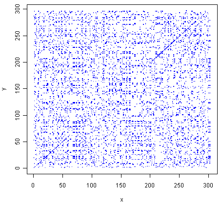
As in Q1, you can see that there is a region of similarity that covers about 60-70 amino acids at the start of the two proteins, then there is a region of similarity from about 210-280 in each of the two proteins.
There are a lot of off-diagonal dots in this picture, because a dot is plotted at every position where the two sequences are identical in one letter (while in Q1, we only plotted a dot at the start of a 10-letter window, where 5 or more out of 10 positions in the window were identical).
The fact that there are so many dots in the picture makes it hard to see the weak region of similarity seen in Q1, from about 85-100 in the two proteins.
Q3.
Adapt the R code in Q2 to write a function that makes a dotplot using a window of size x letters, where a dot is plotted in the first cell of the window if y or more letters compared in that window are identical in the two sequences.
Here is an R function that will do this:
> makeDotPlot3 <- function(seq1,seq2,windowsize,threshold,dotsize=1)
  {
     length1 <- length(seq1)
     length2 <- length(seq2)
     # make a plot:
     x <- 1
     y <- 1
     plot(x,y,ylim=c(1,length2),xlim=c(1,length1),col="white")
     for (i in 1:(length1-windowsize+1))
     {
        word1 <- seq1[i:(i+windowsize)]
        word1b <- c2s(word1)
        for (j in 1:(length2-windowsize+1))
        {
           word2 <- seq2[j:(j+windowsize)]
           word2b <- c2s(word2)
           # count how many identities there are:
           identities <- 0
           for (k in 1:windowsize)
           {
              letter1 <- seq1[(i+k-1)]
              letter2 <- seq2[(j+k-1)]
              if (letter1 == letter2)
              {
                 identities <- identities + 1
              }
           }
           if (identities >= threshold)
           {
              # add a point to the plot at the position
              for (k in 1:1)
              {
                 points(x=(i+k-1),(y=j+k-1),cex=dotsize,col="blue",pch=7)
              }
           }
        }
     }
     print(paste("FINISHED NOW"))
  }
Q4.
Use the dotPlot() function in the SeqinR R package to make a dotplot of rabies virus phosphoprotein and Mokola virus phosphoprotein, using a window size of 3 and a threshold of 3. Use your own R function from Q3 to make a dotplot of rabies virus phosphoprotein and Mokola virus phosphoprotein, using a windowsize (x) of 3 and a threshold (y) of 3. Are the two plots similar or different, and can you explain why?
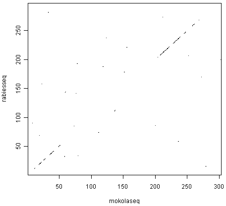
We can use the dotPlot() function from SeqinR to make a dotplot of the rabies and Mokola virus phosphoproteins, using a window size of 3 and a threshold of 3, by typing:
> dotPlot(mokolaseq,rabiesseq,wsize=3,nmatch=3)
We can also use our function makeDotPlot3 to make a dotplot of the rabies and Mokola virus proteins, using a window size of 3 and a threshold of 3:
> makeDotPlot3(mokolaseq,rabiesseq,windowsize=3,threshold=3,dotsize=0.1)
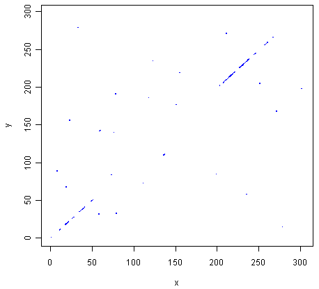
The two pictures are the same, as they should be, as both are plotting a dot in the first position of a 3-letter window if all 3 letters in that window are identical in the two sequences.
Q5.
Write an R function to calculate an unrooted phylogenetic tree with bootstraps, using the minimum evolution method.
We can adjust the function unrootedNJtree, which uses the neighbour-joining method, as it calls the function “nj()” to build a tree.
You can search for R functions that build a tree using minimum evolution method by typing:
> help.search("evolution")
  ape::fastme                Tree Estimation Based on the Minimum Evolution
                             Algorithm
We find that there is a function “fastme()” in the Ape package to build a tree using the minimum evolution method.
You can view the help page for this function by typing ‘help(“fastme”)’. If you do this, you will see that it can be run by typing fastme.bal() or fastme.ols(), which are two different versions of the minimum evolution function.
Thus, we can adapt the unrootedNJtree to make a function that builds a tree using minimum evolution, by using “fastme.bal()” instead of “nj()”:
> unrootedMEtree <- function(alignment,type)
  {
     # load the ape and seqinR packages:
     require("ape")
     require("seqinr")
     # define a function for making a tree:
     makemytree <- function(alignmentmat)
     {
        alignment <- ape::as.alignment(alignmentmat)
        if      (type == "protein")
        {
           mydist <- dist.alignment(alignment)
        }
        else if (type == "DNA")
        {
           alignmentbin <- as.DNAbin(alignment)
           mydist <- dist.dna(alignmentbin)
        }
        mytree <- fastme.bal(mydist)
        mytree <- makeLabel(mytree, space="") # get rid of spaces in tip names.
        return(mytree)
     }
     # infer a tree
     mymat  <- as.matrix.alignment(alignment)
     mytree <- makemytree(mymat)
     # bootstrap the tree
     myboot <- boot.phylo(mytree, mymat, makemytree)
     # plot the tree:
     plot.phylo(mytree,type="u")   # plot the unrooted phylogenetic tree
     nodelabels(myboot,cex=0.7)    # plot the bootstrap values
     mytree$node.label <- myboot   # make the bootstrap values be the node labels
     return(mytree)
  }
Contact
I will be grateful if you will send me (Avril Coghlan) corrections or suggestions for improvements to my email address alc@sanger.ac.uk
License
The content in this book is licensed under a Creative Commons Attribution 3.0 License.