DNA Sequence Statistics (2)¶

A little more introduction to R¶

In the chapter on How to install R, you learnt about variables in R, such as scalars, vectors, and lists. You also learnt how to use functions to carry out operations on variables, for example, using the log10() function to calculate the log to the base 10 of a scalar variable x, or using the mean() function to calculate the average of the values in a vector variable myvector:

> x <- 100
> log10(x)
[1] 2
> myvector <- c(30,16,303,99,11,111)
> mean(myvector)
[1] 95

You also learnt that you can extract an element of a vector by typing the vector name with the index of that element given in square brackets. For example, to get the value of the 3rd element in the vector myvector, we type:

> myvector[3]
[1] 303

A useful function in R is the seq() function, which can be used to create a sequence of numbers that run from a particular number to another particular number. For example, if we want to create the sequence of numbers from 1-100 in steps of 1 (ie. 1, 2, 3, 4, ... 97, 98, 99, 100), we can type:

> seq(1, 100, by = 1)
   1   2   3   4   5   6   7   8   9  10  11  12  13  14  15  16  17  18
 [19]  19  20  21  22  23  24  25  26  27  28  29  30  31  32  33  34  35  36
 [37]  37  38  39  40  41  42  43  44  45  46  47  48  49  50  51  52  53  54
 [55]  55  56  57  58  59  60  61  62  63  64  65  66  67  68  69  70  71  72
 [73]  73  74  75  76  77  78  79  80  81  82  83  84  85  86  87  88  89  90
 [91]  91  92  93  94  95  96  97  98  99 100

We can change the step size by altering the value of the “by” argument given to the function seq(). For example, if we want to create a sequence of numbers from 1-100 in steps of 2 (ie. 1, 3, 5, 7, ... 97, 99), we can type:

> seq(1, 100, by = 2)
 [1]  1  3  5  7  9 11 13 15 17 19 21 23 25 27 29 31 33 35 37 39 41 43 45 47 49
[26] 51 53 55 57 59 61 63 65 67 69 71 73 75 77 79 81 83 85 87 89 91 93 95 97 99

In R, just as in programming languages such as Python, it is possible to write a for loop to carry out the same command several times. For example, if we want to print out the square of each number between 1 and 10, we can write the following for loop:

> for (i in 1:10) { print (i*i) }
[1] 1
[1] 4
[1] 9
[1] 16
[1] 25
[1] 36
[1] 49
[1] 64
[1] 81
[1] 100

In the for loop above, the variable i is a counter for the number of cycles through the loop. In the first cycle through the loop, the value of i is 1, and so i * i =1 is printed out. In the second cycle through the loop, the value of i is 2, and so i * i =4 is printed out. In the third cycle through the loop, the value of i is 3, and so i * i =9 is printed out. The loop continues until the value of i is 10. In the tenth cycle through the loop, the value of i is 10, and so i * i =100 is printed out.

Note that the commands that are to be carried out at each cycle of the for loop must be enclosed within curly brackets (“{” and “}”).

You can also give a for loop a vector of numbers containing the values that you want the counter i to take in subsequent cycles. For example, you can make a vector avector containing the numbers 2, 9, 100, and 133, and write a for loop to print out the square of each number in vector avector:

> avector <- c(2, 9, 100, 133)
> for (i in avector) { print (i*i) }
[1] 4
[1] 81
[1] 10000
[1] 17689

How can we use a for loop to print out the square of every second number between 1 and 10? The answer is to use the seq() function to tell the for loop to take every second number between 1 and 10:

> for (i in seq(1, 10, by = 2)) { print (i*i) }
[1] 1
[1] 9
[1] 25
[1] 49
[1] 81

In the first cycle of this loop, the value of i is 1, and so i * i =1 is printed out. In the second cycle through the loop, the value of i is 3, and so i * i =9 is printed out. The loop continues until the value of i is 9. In the fifth cycle through the loop, the value of i is 9, and so i * i =81 is printed out.

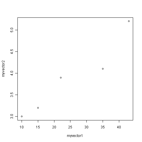
R allows the production of a variety of plots, including scatterplots, histograms, piecharts, and boxplots. For example, if you have two vectors of numbers myvector1 and myvector2, you can plot a scatterplot of the values in myvector1 against the values in myvector2 using the plot() function. If you want to label the axes on the plot, you can do this by giving the plot() function values for its optional arguments xlab and ylab:

> myvector1 <- c(10, 15, 22, 35, 43)
> myvector2 <- c(3, 3.2, 3.9, 4.1, 5.2)
> plot(myvector1, myvector2, xlab="myvector1", ylab="myvector2")

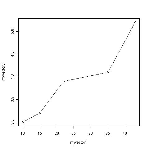
If you look at the help page for the plot() function, you will see that there are lots of optional arguments (inputs) that it can take that. For example, one optional argument is the type argument, that determines the type of the plot. By default, plot() will draw a dot at each data point, but if we set type to be “b”, then it will also draw a line between each subsequent data point:

> plot(myvector1, myvector2, xlab="myvector1", ylab="myvector2", type="b")

We have been using built-in R functions such as mean(), length(), print(), plot(), etc. We can also create our own functions in R to do calculations that you want to carry out very often on different input data sets. For example, we can create a function to calculate the value of 20 plus the square of some input number:

> myfunction <- function(x) { return(20 + (x*x)) }

This function will calculate the square of a number (x), and then add 20 to that value. The return() statement returns the calculated value. Once you have typed in this function, the function is then available for use. For example, we can use the function for different input numbers (eg. 10, 25):

> myfunction(10)
[1] 120
> myfunction(25)
[1] 645

You can view the code that makes up a function by typing its name (without any parentheses). For example, we can try this by typing “myfunction”:

> myfunction
function(x) { return(20 + (x*x)) }

When you are typing R, if you want to, you can write comments by writing the comment text after the “#” sign. This can be useful if you want to write some R commands that other people need to read and understand. R will ignore the comments when it is executing the commands. For example, you may want to write a comment to explain what the function log10() does:

> x <- 100
> log10(x) # Finds the log to the base 10 of variable x.
[1] 2

Reading sequence data with SeqinR¶

In the previous chapter you learnt how to use to search for and download the sequence data for a given NCBI accession from the NCBI Sequence Database, either via the NCBI website or using the getncbiseq() function in R.

For example, you could have downloaded the sequence data for a the DEN-1 Dengue virus sequence (NCBI accession NC_001477), and stored it on a file on your computer (eg. “den1.fasta”).

Once you have downloaded the sequence data for a particular NCBI accession, and stored it on a file on your computer, you can then read it into R by using read.fasta function from the SeqinR R package. For example, if you have stored the DEN-1 Dengue virus sequence in a file “den1.fasta”, you can type:

> library("seqinr")                           # Load the SeqinR package.
> dengue <- read.fasta(file = "den1.fasta")   # Read in the file "den1.fasta".
> dengueseq <- dengue[[1]]                    # Put the sequence in a vector called "dengueseq".

Once you have retrieved a sequence from the NCBI Sequence Database and stored it in a vector variable such as dengueseq in the example above, it is possible to extract subsequence of the sequence by type the name of the vector (eg. dengueseq) followed by the square brackets containing the indices for those nucleotides. For example, to obtain nucleotides 452-535 of the DEN-1 Dengue virus genome, we can type:

> dengueseq[452:535]
 [1] "c" "g" "a" "g" "g" "g" "g" "g" "a" "g" "a" "g" "c" "c" "g" "c" "a" "c" "a"
[20] "t" "g" "a" "t" "a" "g" "t" "t" "a" "g" "c" "a" "a" "g" "c" "a" "g" "g" "a"
[39] "a" "a" "g" "a" "g" "g" "a" "a" "a" "a" "t" "c" "a" "c" "t" "t" "t" "t" "g"
[58] "t" "t" "t" "a" "a" "g" "a" "c" "c" "t" "c" "t" "g" "c" "a" "g" "g" "t" "g"
[77] "t" "c" "a" "a" "c" "a" "t" "g"

Local variation in GC content¶

In the previous chapter, you learnt that to find out the GC content of a genome sequence (percentage of nucleotides in a genome sequence that are Gs or Cs), you can use the GC() function in the SeqinR package. For example, to find the GC content of the DEN-1 Dengue virus sequence that we have stored in the vector dengueseq, we can type:

> GC(dengueseq)
[1] 0.4666977

The output of the GC() is the fraction of nucleotides in a sequence that are Gs or Cs, so to convert it to a percentage we need to multiply by 100. Thus, the GC content of the DEN-1 Dengue virus genome is about 0.467 or 46.7%.

Although the GC content of the whole DEN-1 Dengue virus genome sequence is about 46.7%, there is probably local variation in GC content within the genome. That is, some regions of the genome sequence may have GC contents quite a bit higher than 46.7%, while some regions of the genome sequence may have GC contents that are quite a big lower than 46.7%. Local fluctuations in GC content within the genome sequence can provide different interesting information, for example, they may reveal cases of horizontal transfer or reveal biases in mutation.

If a chunk of DNA has moved by horizontal transfer from the genome of a species with low GC content to a species with high GC content, the chunk of horizontally transferred DNA could be detected as a region of unusually low GC content in the high-GC recipient genome.

On the other hand, a region unusually low GC content in an otherwise high-GC content genome could also arise due to biases in mutation in that region of the genome, for example, if mutations from Gs/Cs to Ts/As are more common for some reason in that region of the genome than in the rest of the genome.

A sliding window analysis of GC content¶

In order to study local variation in GC content within a genome sequence, we could calculate the GC content for small chunks of the genome sequence. The DEN-1 Dengue virus genome sequence is 10735 nucleotides long. To study variation in GC content within the genome sequence, we could calculate the GC content of chunks of the DEN-1 Dengue virus genome, for example, for each 2000-nucleotide chunk of the genome sequence:

> GC(dengueseq[1:2000])      # Calculate the GC content of nucleotides 1-2000 of the Dengue genome
[1] 0.465
> GC(dengueseq[2001:4000])   # Calculate the GC content of nucleotides 2001-4000 of the Dengue genome
[1] 0.4525
> GC(dengueseq[4001:6000])   # Calculate the GC content of nucleotides 4001-6000 of the Dengue genome
[1] 0.4705
> GC(dengueseq[6001:8000])   # Calculate the GC content of nucleotides 6001-8000 of the Dengue genome
[1] 0.479
> GC(dengueseq[8001:10000])  # Calculate the GC content of nucleotides 8001-10000 of the Dengue genome
[1] 0.4545
> GC(dengueseq[10001:10735]) # Calculate the GC content of nucleotides 10001-10735 of the Dengue genome
[1] 0.4993197

From the output of the above calculations, we see that the region of the DEN-1 Dengue virus genome from nucleotides 1-2000 has a GC content of 46.5%, while the region of the Dengue genome from nucleotides 2001-4000 has a GC content of about 45.3%. Thus, there seems to be some local variation in GC content within the Dengue genome sequence.

Instead of typing in the commands above to tell R to calculate the GC content for each 2000-nucleotide chunk of the DEN-1 Dengue genome, we can use a for loop to carry out the same calculations, but by typing far fewer commands. That is, we can use a for loop to take each 2000-nucleotide chunk of the DEN-1 Dengue virus genome, and to calculate the GC content of each 2000-nucleotide chunk. Below we will explain the following for loop that has been written for this purpose:

> starts <- seq(1, length(dengueseq)-2000, by = 2000)
> starts
[1]    1 2001 4001 6001 8001
> n <- length(starts)    # Find the length of the vector "starts"
> for (i in 1:n) {
        chunk <- dengueseq[starts[i]:(starts[i]+1999)]
        chunkGC <- GC(chunk)
        print (chunkGC)
     }
[1] 0.465
[1] 0.4525
[1] 0.4705
[1] 0.479
[1] 0.4545

The command “starts <- seq(1, length(dengueseq)-2000, by = 2000)” stores the result of the seq() command in the vector starts, which contains the values 1, 2001, 4001, 6001, and 8001.

We set the variable n to be equal to the number of elements in the vector starts, so it will be 5 here, since the vector starts contains the five elements 1, 2001, 4001, 6001 and 8001. The line “for (i in 1:n)” means that the counter i will take values of 1-5 in subsequent cycles of the for loop. The for loop above is spread over several lines. However, R will not execute the commands within the for loop until you have typed the final “}” at the end of the for loop and pressed “Return”.

Each of the three commands within the for loop are carried out in each cycle of the loop. In the first cycle of the loop, i is 1, the vector variable chunk is used to store the region from nucleotides 1-2000 of the Dengue virus sequence, the GC content of that region is calculated and stored in the variable chunkGC, and the value of chunkGC is printed out.

In the second cycle of the loop, i is 2, the vector variable chunk is used to store the region from nucleotides 2001-4000 of the Dengue virus sequence, the GC content of that region is calculated and stored in the variable chunkGC, and the value of chunkGC is printed out. The loop continues until the value of i is 5. In the fifth cycle through the loop, the value of i is 5, and so the GC content of the region from nucleotides 8001-10000 is printed out.

Note that we stop the loop when we are looking at the region from nucleotides 8001-10000, instead of continuing to another cycle of the loop where the region under examiniation would be from nucleotides 10001-12000. The reason for this is because the length of the Dengue virus genome sequence is just 10735 nucleotides, so there is not a full 2000-nucleotide region from nucleotide 10001 to the end of the sequence at nucleotide 10735.

The above analysis of local variation in GC content is what is known as a sliding window analysis of GC content. By calculating the GC content in each 2000-nucleotide chunk of the Dengue virus genome, you are effectively sliding a 2000-nucleotide window along the DNA sequence from start to end, and calculating the GC content in each non-overlapping window (chunk of DNA).

Note that this sliding window analysis of GC content is a slightly simplified version of the method usually carried out by bioinformaticians. In this simplified version, we have calculated the GC content in non-overlapping windows along a DNA sequence. However, it is more usual to calculate GC content in overlapping windows along a sequence, although that makes the code slightly more complicated.

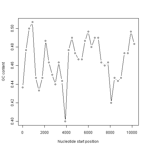
A sliding window plot of GC content¶

It is common to use the data generated from a sliding window analysis to create a sliding window plot of GC content. To create a sliding window plot of GC content, you plot the local GC content in each window of the genome, versus the nucleotide position of the start of each window. We can create a sliding window plot of GC content by typing:

> starts <- seq(1, length(dengueseq)-2000, by = 2000)
> n <- length(starts)    # Find the length of the vector "starts"
> chunkGCs <- numeric(n) # Make a vector of the same length as vector "starts", but just containing zeroes
> for (i in 1:n) {
        chunk <- dengueseq[starts[i]:(starts[i]+1999)]
        chunkGC <- GC(chunk)
        print(chunkGC)
        chunkGCs[i] <- chunkGC
     }
> plot(starts,chunkGCs,type="b",xlab="Nucleotide start position",ylab="GC content")

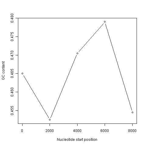
In the code above, the line “chunkGCs <- numeric(n)” makes a new vector chunkGCs which has the same number of elements as the vector starts (5 elements here). This vector chunkGCs is then used within the for loop for storing the GC content of each chunk of DNA.

After the loop, the vector starts can be plotted against the vector chunkGCs using the plot() function, to get a plot of GC content against nucleotide position in the genome sequence. This is a sliding window plot of GC content.

You may want to use the code above to create sliding window plots of GC content of different species’ genomes, using different windowsizes. Therefore, it makes sense to write a function to do the sliding window plot, that can take the windowsize that the user wants to use and the sequence that the user wants to study as arguments (inputs):

> slidingwindowplot <- function(windowsize, inputseq)
{
   starts <- seq(1, length(inputseq)-windowsize, by = windowsize)
   n <- length(starts)    # Find the length of the vector "starts"
   chunkGCs <- numeric(n) # Make a vector of the same length as vector "starts", but just containing zeroes
   for (i in 1:n) {
        chunk <- inputseq[starts[i]:(starts[i]+windowsize-1)]
        chunkGC <- GC(chunk)
        print(chunkGC)
        chunkGCs[i] <- chunkGC
   }
   plot(starts,chunkGCs,type="b",xlab="Nucleotide start position",ylab="GC content")
}

This function will make a sliding window plot of GC content for a particular input sequence inputseq specified by the user, using a particular windowsize windowsize specified by the user. Once you have typed in this function once, you can use it again and again to make sliding window plots of GC contents for different input DNA sequences, with different windowsizes. For example, you could create two different sliding window plots of the DEN-1 Dengue virus genome sequence, using windowsizes of 3000 and 300 nucleotides, respectively:

> slidingwindowplot(3000, dengueseq)

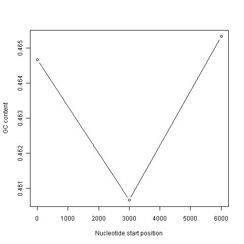
> slidingwindowplot(300, dengueseq)

Over-represented and under-represented DNA words¶

In the previous chapter, you learnt that the count() function in the SeqinR R package can calculate the frequency of all DNA words of a certain length in a DNA sequence. For example, if you want to know the frequency of all DNA words that are 2 nucleotides long in the Dengue virus genome sequence, you can type:

> count(dengueseq, 2)
 aa   ac   ag   at   ca   cc   cg   ct   ga   gc   gg   gt   ta   tc   tg   tt
1108  720  890  708  901  523  261  555  976  500  787  507  440  497  832  529

It is interesting to identify DNA words that are two nucleotides long (“dinucleotides”, ie. “AT”, “AC”, etc.) that are over-represented or under-represented in a DNA sequence. If a particular DNA word is over-represented in a sequence, it means that it occurs many more times in the sequence than you would have expected by chance. Similarly, if a particular DNA word is under-represented in a sequence, it means it occurs far fewer times in the sequence than you would have expected.

A statistic called ρ (Rho) is used to measure how over- or under-represented a particular DNA word is. For a 2-nucleotide (dinucleotide) DNA word ρ is calculated as:

ρ(xy) = f_xy/(f_x*f_y),

where f_xy and f_x are the frequencies of the DNA words xy and x in the DNA sequence under study. For example, the value of ρ for the DNA word “TA” can be calculated as: ρ(TA) = f_TA/(f_T* f_A), where f_TA, f_T and f_A are the frequencies of the DNA words “TA”, “T” and “A” in the DNA sequence.

The idea behind the ρ statistic is that, if a DNA sequence had a frequency f_x of a 1-nucleotide DNA word x, and a frequency f_y of a 1-nucleotide DNA word y, then we expect the frequency of the 2-nucleotide DNA word xy to be f_x* f_y. That is, the frequencies of the 2-nucleotide DNA words in a sequence are expected to be equal the products of the specific frequencies of the two nucleotides that compose them. If this were true, then ρ would be equal to 1. If we find that ρ is much greater than 1 for a particular 2-nucleotide word in a sequence, it indicates that that 2-nucleotide word is much more common in that sequence than expected (ie. it is over-represented).

For example, say that your input sequence has only 5% Ts (ie. f_T = 0.05). In a random DNA sequence with 5% Ts, you would expect to see the word “TT” very infrequently. In fact, we would only expect 0.05 * 0.05=0.0025 (0.25%) of 2-nucleotide words to be TTs (ie. we expect f_TT = f_T* f_T). This is because Ts are rare, so they are expected to be adjacent to each other very infrequently if the few Ts are randomly scattered throughout the DNA. Therefore, if you see lots of TT 2-nucleotide words in your real input sequence (eg. f_TT = 0.3, so ρ = 0.3/0.0025 = 120), you would suspect that natural selection has acted to increase the number of occurrences of the TT word in the sequence (presumably because it has some beneficial biological function).

To find over-represented and under-represented DNA words that are 2 nucleotides long in the DEN-1 Dengue virus sequence, we can calculate the ρ statistic for each 2-nucleotide word in the sequence. For example, given the number of occurrences of the individual nucleotides A, C, G and T in the Dengue sequence, and the number of occurrences of the DNA word GC in the sequence (500, from above), we can calculate the value of ρ for the 2-nucleotide DNA word “GC”, using the formula ρ(GC) = f_GC/(f_G * f_C), where f_GC, f_G and f_C are the frequencies of the DNA words “GC”, “G” and “C” in the DNA sequence:

> count(dengueseq, 1) # Get the number of occurrences of 1-nucleotide DNA words
    a     c     g     t
   3426 2240 2770 2299
> 2770/(3426+2240+2770+2299) # Get fG
[1] 0.2580345
> 2240/(3426+2240+2770+2299) # Get fC
[1] 0.2086633
> count(dengueseq, 2) # Get the number of occurrences of 2-nucleotide DNA words
  aa   ac   ag   at   ca   cc   cg   ct   ga   gc   gg   gt   ta   tc   tg   tt
 1108  720  890  708  901  523  261  555  976  500  787  507  440  497  832  529
> 500/(1108+720+890+708+901+523+261+555+976+500+787+507+440+497+832+529) # Get fGC
[1] 0.04658096
> 0.04658096/(0.2580345*0.2086633) # Get rho(GC)
[1] 0.8651364

We calculate a value of ρ(GC) of approximately 0.865. This means that the DNA word “GC” is about 0.865 times as common in the DEN-1 Dengue virus sequence than expected. That is, it seems to be slightly under-represented.

Note that if the ratio of the observed to expected frequency of a particular DNA word is very low or very high, then we would suspect that there is a statistical under-representation or over-representation of that DNA word. However, to be sure that this over- or under-representation is statistically significant, we would need to do a statistical test. We will not deal with the topic of how to carry out the statistical test here.

Summary¶

In this chapter, you will have learnt to use the following R functions:

seq() for creating a sequence of numbers
print() for printing out the value of a variable
plot() for making a plot (eg. a scatterplot)
numeric() for making a numeric vector of a particular length
function() for making a function

All of these functions belong to the standard installation of R. You also learnt how to use for loops to carry out the same operation again and again, each time on different inputs.

Links and Further Reading¶

Some links are included here for further reading.

For background reading on DNA sequence statistics, it is recommended to read Chapter 1 of Introduction to Computational Genomics: a case studies approach by Cristianini and Hahn (Cambridge University Press; www.computational-genomics.net/book/).

For more in-depth information and more examples on using the SeqinR package for sequence analysis, look at the SeqinR documentation, http://pbil.univ-lyon1.fr/software/seqinr/doc.php?lang=eng.

There is also a very nice chapter on “Analyzing Sequences”, which includes examples of using SeqinR for sequence analysis, in the book Applied statistics for bioinformatics using R by Krijnen (available online at cran.r-project.org/doc/contrib/Krijnen-IntroBioInfStatistics.pdf).

For a more in-depth introduction to R, a good online tutorial is available on the “Kickstarting R” website, cran.r-project.org/doc/contrib/Lemon-kickstart.

There is another nice (slightly more in-depth) tutorial to R available on the “Introduction to R” website, cran.r-project.org/doc/manuals/R-intro.html.

Acknowledgements¶

Thank you to Noel O’Boyle for helping in using Sphinx, http://sphinx.pocoo.org, to create this document, and github, https://github.com/, to store different versions of the document as I was writing it, and readthedocs, http://readthedocs.org/, to build and distribute this document.

Many of the ideas for the examples and exercises for this chapter were inspired by the Matlab case studies on Haemophilus influenzae (www.computational-genomics.net/case_studies/haemophilus_demo.html) and Bacteriophage lambda (http://www.computational-genomics.net/case_studies/lambdaphage_demo.html) from the website that accompanies the book Introduction to Computational Genomics: a case studies approach by Cristianini and Hahn (Cambridge University Press; www.computational-genomics.net/book/).

Thank you to Jean Lobry and Simon Penel for helpful advice on using the SeqinR package.

Contact¶

I will be grateful if you will send me (Avril Coghlan) corrections or suggestions for improvements to my email address alc@sanger.ac.uk

License¶

The content in this book is licensed under a Creative Commons Attribution 3.0 License.

Exercises¶

Answer the following questions, using the R package. For each question, please record your answer, and what you typed into R to get this answer.

Model answers to the exercises are given in Answers to the exercises on DNA Sequence Statistics (2).

Q1. Draw a sliding window plot of GC content in the DEN-1 Dengue virus genome, using a window size of 200 nucleotides. Do you see any regions of unusual DNA content in the genome (eg. a high peak or low trough)?: Make a sketch of each plot that you draw. At what position (in base-pairs) in the genome is there the largest change in local GC content (approximate position is fine here)? Compare the sliding window plots of GC content created using window sizes of 200 and 2000 nucleotides. How does window size affect your ability to detect differences within the Dengue virus genome?
Q2. Draw a sliding window plot of GC content in the genome sequence for the bacterium Mycobacterium leprae strain TN (accession NC_002677) using a window size of 20000 nucleotides. Do you see any regions of unusual DNA content in the genome (eg. a high peak or low trough)?: Make a sketch of each plot that you draw. Write down the approximate nucleotide position of the highest peak or lowest trough that you see. Why do you think a window size of 20000 nucleotides was chosen? What do you see if you use a much smaller windowsize (eg. 200 nucleotides) or a much larger windowsize (eg. 200,000 nucleotides)?
Q3. Write a function to calculate the AT content of a DNA sequence (ie. the fraction of the nucleotides in the sequence that are As or Ts). What is the AT content of the Mycobacterium leprae TN genome?: Hint: use the function count() to make a table containing the number of As, Gs, Ts and Cs in the sequence. Remember that function count() produces a table object, and you can access the elements of a table object using double square brackets. Do you notice a relationship between the AT content of the Mycobacterium leprae TN genome, and its GC content?
Q4. Write a function to draw a sliding window plot of AT content. Use it to make a sliding window plot of AT content along the Mycobacterium leprae TN genome, using a windowsize of 20000 nucleotides. Do you notice any relationship between the sliding window plot of GC content along the Mycobacterium leprae genome, and the sliding window plot of AT content?: Make a sketch of the plot that you draw.
Q5. Is the 3-nucleotide word GAC GC over-represented or under-represented in the Mycobacterium leprae TN genome sequence?: What is the frequency of this word in the sequence? What is the expected frequency of this word in the sequence? What is the ρ (Rho) value for this word? How would you figure out whether there is already an R function to calculate ρ (Rho)? Is there one that you could use?

Table Of Contents

Previous topic

Next topic

This Page